Physics Baseline

This section will give a short summary of Dark matter and the basic physics behind the analysis we will go through in the school.

Dark Matter

One of the open questions of modern-day physics is related to the properties of DM. The existence of dark matter is implied through several astrophysical obseervations including galactic rotation curves, gravitational lensing, and the cosmic microwave background.

Weakly interacting massive particles (WIMPs) are a hypothetical proposed candidate for DM. While there is no rigid definition of what constitutes a WIMP, they are generally new elemental particles that interact with the SM as weak or weaker than the weak nuclear force.

In spite of the abundance of DM, its nature remains unknown. This mystery is the subject of an active experimental program to search for dark matter particles, including direct-detection experiments that search for interactions of ambient DM with ordinary matter, indirect-detection experiments that search for the products of self-annihilation of DM in outer space, and searches at accelerators and colliders that attempt to create DM in the laboratory. The figure below shows a diagram showing the different detection techniques used to search for evidence of DM. The arrows indicate the flow of time for the different interactions, yielding a different combination of SM and DM particles.

We will focus on DM produced at the LHC, but brief descriptions of Direct and Indirect detection are explained below.

Simplified Dark Matter at CMS

With DM particles in the GeV and TeV mass range, experiments at the LHC may be able to detect DM particles produced in the proton-proton (pp) collisions. Because DM will have negligible interactions with the SM, the DM particles would not be detected by typical detector systems, instead appearing as large amounts of missing transverse momentum. The search presented in this thesis considers a “mono-Z” scenario where a Z boson, produced in pp collisions, recoils against DM or other beyond the standard model (BSM) invisible particles. The Z boson subsequently decays into two charged leptons. This school focuses on this dilepton signature, and the accompanying undetected particles contribute to missing transverse momentum.

For this school we will examine a set of simplified models for DM production. These models describe the phenomenology of DM production at the LHC with a small number of parameters and provide a standard for comparing and combining results from different search channels. Four simple ultraviolet-complete models that contain a massive mediator exchanged in the s-channel are considered. For these models, the mediator (either a scalar, psuedoscalar, vector, or axial-vector) couples directly to quarks and the DM particle χ, where χ is assumed to be a Dirac fermion. Here, the couplings to Standard model quarks, the coupling to dark matter and the mediator mass are all tunable parameters leading to a wide variety of kinematic possibilities.

Direct Detection

Direct detection experiments attempt to collect direct evidence for the presence of dark matter through the observation of low energy elastic collisions between DM particles and atomic nuclei. As DM particles pass through the Earth, they can collide with a nucleus that will emit energy (on the order of keV) as scintillation light or as phonons as they pass through a sensitive apparatus. These apparatuses are often buried deep underground in order to reduce the background, specifically from cosmic rays. Direct detection experiments primarily use either cryogenic detectors, operating at temperatures below 100 mK, or liquid detector technologies that detect scintillation originating from a collision with a noble liquid or metalloid, such as a xenon, argon or germanium nuclei.

While no evidence for DM has been found from direct detection experiments, several experiments have placed limits on the nucleon cross sections of DM interactions. Some example of recent limits from noble liquid experiments include recent results from the XENON1T, the Large Underground Xenon (LUX), the DarkSide-50 and the PandaX-ll experiments. Results from cryogenic detectors include the CRESST-III, the CDMS and SuperCDMS experiments, while additional results from bubble chambers include the PICO-60 and PICO-2L experiments.

Indirect Detection

Indirect detection experiments aim to search for particles originating from the self-annihilation or decay of dark matter particles in the universe. In regions of high dark matter density, DM particles could collide, annihilate and produce SM particles, either in particle-antiparticle pairs or through high energy photons (gamma rays). If the DM particles are inherently unstable, they could also decay into SM particles. Both of these processes have potential to be detected indirectly through observations of excess amounts of gamma rays, antiprotons or positrons.

In addition to self-annihilation in space, excess neutrinos from stars such as our sun may indicate the presence of DM. As DM particles pass through massive objects, they may scatter off SM particles, losing energy. This could cause an accumulation of DM particles at the center of massive objects. If these DM self-annihilate, they could be observed as an excess amount of high energy neutrinos originating from these bodies.

Several experiments are already searching for these distinct signatures. The Fermi-LAT looks for excess gamma rays. The PAMELA experiment has observed an excess of positrons, that could be caused from DM particle annihilation of from pulsars. The PAMELA experiment also searched for excess antiprotons but did not observe any excess. The Alpha Magnetic Spectrometer (AMS-02), located on the international space station, also indicated an excess of high energy positrons. The IceCube and Super-Kamiokande neutrino observatories have presented constraints on the annihilation cross section from searches for an excess neutrino flux.

---

Framework

This section will guide you through some of the details of the framework.

Install the Mono-Z framework

Install framework: Installl this framework in eos area

ssh -L localhost:8NNN:localhost:8NNN lxplus.cern.ch

Choose the port above (like 8099) and match it in the command below to start a jupyter session. You will need to copy the url from the following.

git clone git@github.com:shachary0201/CMSDAS-MonoZ-Tutorial-2025-IITH.git
cd CMSDAS-MonoZ-Tutorial-2025-IITH
sh bootstrap.sh

To start the singularity environment.

./shell

If you want to start a jupyter session inside this singularity use below with the same port through which you have logged into lxplus

jupyter lab --no-browser --port 8NNN

List of backgrounds

Main backgrounds:

• ZZ (Irreducible)
• WZ (Irreducible)
• top pair production
• WW
• Drell-Yan (DY)
• Triboson

It’s important to define control regions to check that our simulation well describes the backgrounds. We use 4 main backgrounds for this analysis

• 4 lepton control region (Normalization of ZZ)
• 3 lepton control region (Normalization of WZ)
• Nonresonant control region (Normalization for WW and top pair production)
• Low pTmiss sideband region (Normalization for DY)

Look at Trees introduction

Install the Mono-Z analysis code (Commands above):

NTuples for 2016 are stored the EOS space we can use:

Exit from singulariy open the root file in the new tab using lxplus

/eos/user/c/cmsdas/long-exercises/MonoZ/

An example of how to look at a sample root file:

root -l /eos/user/c/cmsdas/long-exercises/MonoZ/CMSDAS_NTuples/ZZTo2L2Nu_13TeV_powheg_pythia8_ext1/tree_0.root

Since root is not installed inside singularity, therfore we need to perform root outside the singularity This will open a root session where you can look at a sample file quickly in an interactive session:

new TBrowser

If u donot have access to eos, we kept few files in public area you can use them

/afs/cern.ch/user/s/shachary/public/rootfilesmonoX

Each root file contains a TTree called “Events”. The trees have many branches, that correspond to single physics variables. They may be have:

• single floats, for example variables characterising the whole event
• vectors of variables, for example variables related to a particle type, as pT of the electrons. For these cases, also an an integer defining the size of the vector is present for example “nLepton”. The variables are then defined as Collection_variable (e.g. Electron_pt[0]) and the indexing is such that the objects are pT ordered (Object_pt[0] > Object_pt[1] > Object_pt[2] > …)

The general strategy is the following:

events from the data are required to pass the trigger selections described above (with arbitration described in the following

in the Monte Carlo simulations (MC) the trigger selection is missing, and it is emulated weighing events with coefficients that mimic the trigger efficiency effect. Weights are used also to correct any residual differences observed between data and MC. All the weights used have to be multiplied, to produce a total weighting factor.

More information about nanoAOD trees can be found at in the documentation in NanoAOD

Some variables have been added in the aforementioned post-processing, for example the combined variable “invariant mass of the two leading pT leptons”, Z_mass. If you want to learn more and discover how the variables are built, check here : Producer

Lets look at some ROOT commands to make some simple histograms.

Lets start by just looking at the pTmiss distribution directly:

Events->Scan("met_pt","","")

Does it make sense? Ok, let’s add some simple selections. Let’s look at the pTmiss but only for events with 2 electrons with pT>20 GeV:

Events->Scan("met_pt","nElectron==2 && Electron_pt[0]>20. && Electron_pt[1]>20.","")

Try to look through the ROOT file and do the same thing as above except for muons. Do they look similar? These commands are very simple but they are often a good way to check things quickly! These Trees also contain several variables that we have added specifically for this analysis. These variables are explained in the next section but one of the most important ones is the mass of the Z boson candidate (Z_mass). Find a sample with a leptonically decaying Z boson (ZZ) and look at this variable.

Events->Scan("Z_mass")

We can select clean Z boson

Events->Scan("Z_mass", "Z_mass > 80 && Z_mass < 100")

Find a sample that doesn’t have a Z (ttbar). What does it look like there?

Another quick and potentially useful command is to look at both the phi and eta at the same time. Let’s look at this for the Z boson candidate:

Since Draw is slow in lxplus, it would be good to download the file as illustrated in the previous section and than draw it

Events->Draw("Z_eta:Z_phi","","colz")

---

Trees Content

Several combined kinematic variables are precomputed in the ntuples. Key variables used in the signal region are listed below:

Name in NTuple	Description
Z_pt	Transverse momentum of the Z boson candidate
Z_mass	Invariant mass of the Z boson candidate
delta_phi_ll	Δφ between the two leading leptons
delta_R_ll	ΔR between the two leading leptons
sca_balance	Ratio of (MET - Z momentum) over their sum; small for recoiling systems
delta_phi_ZMet	Δφ between the Z boson candidate and the missing transverse momentum
delta_phi_j_met	Δφ between the jet candidate and the missing transverse momentum
met_pt	Magnitude of the missing transverse momentum (Type-1 PF MET with NVtx corrections)
MT	Transverse mass of the dilepton + MET system:

---

Welcome to CMSDAS

Welcome to the mono-Z long exercise for CMSDAS. This site will guide you through the exercise and give you examples on how to use the code.

Facilitators

IIT HYDERABAD 2025

• Bhawna Gomber
• Varun Sharma
• Shriniketan Acharya

LPC 2025

• Daniel Fernando Guerrero Ibarra
• Nick Manganelli
• Rafey Hashmi
• Richa Sharma
• Tetiana Mazurets
• Matteo Cremonosi

CERN 2024

• Yacine Haddad
• Chad Freer
• Nick Manganelli
• Rafey Hashmi

Long Exercise

The outline of the analysis is explained in a set of slides. The general workflow of the mono-Z analysis is shown below. Due to time constraints, we will focus on the last 3 steps as explained in the exercise section of this guide.

What You Will Do

---

Making Datacards

An important part of an analysis before running combine is the creation of datacards describing the rates, uncertainties and normalizations for the various processes used in the analysis. In this section we will describe what a typical datacard looks like and the various components. Finally we can run our own datacards and see the limits as described in the following section.

Mono Z Datacards

imax * number of categories
jmax * number of samples minus one
kmax * number of nuisance parameters
------------------------------
shapes * * shapes-chBSM2016.root $PROCESS $PROCESS_$SYSTEMATIC
bin           chBSM2016
observation      2236.0
------------------------------
------------------------------
bin                                 chBSM2016      chBSM2016      chBSM2016      chBSM2016      chBSM2016      chBSM2016      chBSM2016
process                             Signal         ZZ             WZ             WW             VVV            TOP            DY
process                             0              1              2              3              4              5              6
rate                                151.785        470.638        352.725        74.218         2.589          280.862        811.159
------------------------------
CMS_BTag_2016            shape      1.000          1.000          1.000          1.000          1.000          1.000          1.000
CMS_EFF_e                shape      1.000          1.000          1.000          1.000          1.000          1.000          1.000
CMS_EFF_m                shape      1.000          1.000          1.000          1.000          1.000          1.000          1.000
CMS_JER_2016             shape      1.000          1.000          1.000          1.000          1.000          1.000          1.000
CMS_JES_2016             shape      1.000          1.000          1.000          1.000          1.000          1.000          1.000
CMS_PU_2016              shape      1.000          1.000          1.000          1.000          1.000          1.000          1.000
CMS_QCDScaleSignal_2016  shape      1.000            -              -              -              -              -              -
CMS_QCDScaleTOP_2016     shape        -              -              -              -              -            1.000            -
CMS_QCDScaleVVV_2016     shape        -              -              -              -            1.000            -              -
CMS_QCDScaleWW_2016      shape        -              -              -            1.000            -              -              -
CMS_QCDScaleWZ_2016      shape        -              -            1.000            -              -              -              -
CMS_QCDScaleZZ_2016      shape        -            1.000            -              -              -              -              -
CMS_RES_e                  lnN      1.005          1.005          1.005          1.005          1.005          1.005          1.005
CMS_RES_m                  lnN      1.005          1.005          1.005          1.005          1.005          1.005          1.005
CMS_Trig_2016            shape      1.000          1.000          1.000          1.000          1.000          1.000          1.000
CMS_Vx_2016              shape      1.000          1.000          1.000          1.000          1.000          1.000          1.000
CMS_lumi_2016              lnN      1.025          1.025          1.025          1.025          1.025          1.025          1.025
CMS_pfire_2016           shape      1.000            -              -              -              -              -              -
EWKWZ                    shape        -              -            1.000            -              -              -              -
EWKZZ                    shape        -            1.000            -              -              -              -              -
PDF_2016                 shape      1.000          1.000          1.000          1.000          1.000          1.000          1.000
UEPS                       lnN      1.020          1.020          1.020          1.020          1.020          1.020          1.020
VVnorm_0_                shape        -            1.000          1.000              -            -              -              -
VVnorm_1_                shape        -            1.000          1.000              -            -              -              -
VVnorm_2_                shape        -            1.000          1.000              -            -              -              -
EMnorm_2016 rateParam chBSM* WW 1 [0.1,10]
DYnorm_2016 rateParam chBSM* DY 1 [0.1,10]
chBSM2016 autoMCStats 0 0 1
EMnorm_2016 rateParam chBSM* TOP 1 [0.1,10]

Understanding the datacards

A counting experiment is a search where we just count the number of events that pass a selection, and compare that number with the event yields expected from the signal and background.

A shape analysis relies not only on the expected event yields for the signals and backgrounds, but also on the distribution of those events in some discriminating variable. This approach is often convenient with respect to a counting experiment, especially when the background cannot be predicted reliably a-priori, since the information from the shape allows a better discrimination between a signal-like and a background-like excess, and provides an in-situ normalization of the background.

The simpler case of shape analysis is the binned one: the observed distribution of the events in data and the expectations from the signal and all backgrounds are provided as histograms, all with the same binning. Mathematically, this is equivalent to just making N counting experiments, one for each bin of the histogram; however, in practice it’s much more convenient to provide the the predictions as histograms directly.

For this kind of analysis, all the information needed for the statistical interpretation of the results is encoded in a simple text file. An example was shown above as the datacard for cards-DMSimp_MonoZLL_Pseudo_500_mxd-1/shapes-chBSM2016.dat. Let’s go through the various components of this datacard and try to understand it.

Channels:

These lines describe the basics of the datacard: the number of channels, physical processes, and systematical uncertainties. Only the first two words (e.g. imax) are interpreted, the rest is a comment.

• imax defines the number of final states analyzed (one in this case, but datacards can also contain multiple channels)
• jmax defines the number of independent physical processes whose yields are provided to the code, minus one (i.e. if you have 2 signal processes and 5 background processes, you should put 6)
• kmax defines the number of independent systematical uncertainties (these can also be set to * or -1 which instruct the code to figure out the number from what’s in the datacard)

You’ll notice that in this datacard these numbers are not filled. This is because this datacard is written specifically for the signal region. The full datacard is written in combined.dat and will show these numbers (too long to show here).

imax * number of categories
jmax * number of samples minus one
kmax * number of nuisance parameters

Processes and Rates

These lines describe the number of observed events in each final state. In this case, there’s a final state, with label chBSM2016 that contains the events in our signal region. The observation is the number of data events in this channel. You will also se the background then split into the different processes. Does the observation seem to match the background estimation? Check the rates to see if they make sense.

shapes * * shapes-chBSM2016.root $PROCESS $PROCESS_$SYSTEMATIC
bin           chBSM2016
observation      2236.0
------------------------------
------------------------------
bin                                 chBSM2016      chBSM2016      chBSM2016      chBSM2016      chBSM2016      chBSM2016      chBSM2016
process                             Signal         ZZ             WZ             WW             VVV            TOP            DY
process                             0              1              2              3              4              5              6
rate                                151.785        470.638        352.725        74.218         2.589          280.862        811.159

Systematic Uncertainties

The next section deals with the uncertainties and normalizations associated with the different yields. The way systematical uncertainties are implemented in the Higgs statistics package is by identifying each independent source of uncertainty, and describing the effect it has on the event yields of the different processes. Each source is identified by a name, and in the statistical model it will be associated with a nuisance parameter.

An individual source of uncertainty can have an effect on multiple processes, also across different channels, and all these effects will be correlated (e.g., the uncertainty on the production cross section for DY will affect the expected event yield for this process in all datacards). While not necessarily problematic for this analysis, the size of the effect doesn’t have to be the same, e.g., a 1% uncertainty on the muon resolution might have a 2% effect on WW→ℓνℓν but a 4% effect on ZZ→4l. Anti-correlations are also possible (e.g., an increase in b-tagging efficiency will simultaneously and coherently increase the signal yield in final states that require tagged b-jets and decrease the signal yield in final states that require no tagged b-jets).

The use of names for each source of uncertainty allows the code to be able to combine multiple datacards recognizing which uncertainties are in common and which are instead separate.

The most common model used for systematical uncertainties is the log-normal distribution, which is identified by the lnN keyword in combine. The distribution is characterized by a parameter κ, and affects the expected event yields in a multiplicative way: a positive deviation of +1σ corresponds to a yield scaled by a factor κ compared to the nominal one, while a negative deviation of -1σ corresponds to a scaling by a factor 1/κ. For small uncertainties, the log-normal is approximately a Gaussian. If Δx/x* is the relative uncertainty on the yield, κ can be set to 1+Δx/x.

We can also consider systematical uncertainties that affect not just the normalization but also the shape of the expected distribution for a process. You should recognize some of the shape based systematics from the histograms earlier. The datacard helps tell combine what systematics are associated with various processes and how they are correlated. For example, the JES are applied to all processes and the uncertainty is correlated among the different processes, while the EWK corrections are only applied to the WZ and the ZZ and are uncorrelated. Additionally, if you are using the full Run-2 dataset you could set correlations among the different years here as well.

CMS_BTag_2016            shape      1.000          1.000          1.000          1.000          1.000          1.000          1.000
CMS_EFF_e                shape      1.000          1.000          1.000          1.000          1.000          1.000          1.000
CMS_EFF_m                shape      1.000          1.000          1.000          1.000          1.000          1.000          1.000
CMS_JER_2016             shape      1.000          1.000          1.000          1.000          1.000          1.000          1.000
CMS_JES_2016             shape      1.000          1.000          1.000          1.000          1.000          1.000          1.000
CMS_PU_2016              shape      1.000          1.000          1.000          1.000          1.000          1.000          1.000
CMS_QCDScaleSignal_2016  shape      1.000            -              -              -              -              -              -
CMS_QCDScaleTOP_2016     shape        -              -              -              -              -            1.000            -
CMS_QCDScaleVVV_2016     shape        -              -              -              -            1.000            -              -
CMS_QCDScaleWW_2016      shape        -              -              -            1.000            -              -              -
CMS_QCDScaleWZ_2016      shape        -              -            1.000            -              -              -              -
CMS_QCDScaleZZ_2016      shape        -            1.000            -              -              -              -              -
CMS_RES_e                  lnN      1.005          1.005          1.005          1.005          1.005          1.005          1.005
CMS_RES_m                  lnN      1.005          1.005          1.005          1.005          1.005          1.005          1.005
CMS_Trig_2016            shape      1.000          1.000          1.000          1.000          1.000          1.000          1.000
CMS_Vx_2016              shape      1.000          1.000          1.000          1.000          1.000          1.000          1.000
CMS_lumi_2016              lnN      1.025          1.025          1.025          1.025          1.025          1.025          1.025
CMS_pfire_2016           shape      1.000            -              -              -              -              -              -
EWKWZ                    shape        -              -            1.000            -              -              -              -
EWKZZ                    shape        -            1.000            -              -              -              -              -
PDF_2016                 shape      1.000          1.000          1.000          1.000          1.000          1.000          1.000
UEPS                       lnN      1.020          1.020          1.020          1.020          1.020          1.020          1.020
VVnorm_0_                shape        -            1.000          1.000              -            -              -              -
VVnorm_1_                shape        -            1.000          1.000              -            -              -              -
VVnorm_2_                shape        -            1.000          1.000              -            -              -              -

Normalizations

The last section handles the single bin normalization factors for the EMU (Top and WW) and the DY region. For this the normalization is allowed to float anywhere between 0.1 and 10.

EMnorm_2016 rateParam chBSM* WW 1 [0.1,10]
DYnorm_2016 rateParam chBSM* DY 1 [0.1,10]
chBSM2016 autoMCStats 0 0 1
EMnorm_2016 rateParam chBSM* TOP 1 [0.1,10]

Take some time to look through the datacards for the other channels (control regions). Do they make sense to you? Can you follow some of the systematics and see why they are applied to certain processes and not to others. What about the correlations? The next step would be to look at the combined.dat which combines all of the signal and control regions. These are much bigger but contain the same information. Does the combined datacard make sense? We will be using this as input to combine so make sure these are clear to you.

Running your own datacards

The code to run the datacards can be see here Datacard.

In here the systematic variations are described here systematic_variations. and the rate params here rate_params.

This will run datacards for every file here Input.

In order to run this code you will need to tell it the region of interest. This can be seen in an example command below: Here we can just run the datacard for the SR and examine the datacard to see if it makes sense. You can examine other Dark Matter models by modifying the input_DAS_2016.yaml. The makecard-boost.py has the systmatics commented out. Feel free to play with these and add them back in.

To make a datacard, please move into datacards directory
cd ../datacards

than

python3 makecard-boost.py --name monoZ --input ./config/input_DAS_2016.yaml --era 2016 --variable met_pt --channel catSignal-0jet

---

Making Histograms

An integral part of understanding physics, is finding ways to display data in a way that can be easily understood. One of the fundamental tools in a physicists toolbelt is the histogram which allows us to show binned data a plethora of different ways. This section will walk you through how to create a histogram using the Mono Z framework.

An Introduction to Making Histograms from Trees

Starting from the NTuples we have introduced, we will make histograms for our Control and Signal regions. We will do these for each file filled with NTuples. This means we will need to run our code over a large number of files. In order to make this easier we will submit the jobs on HT Condor and place the output in another directory. These files will only contain the histograms that we want to look at and will be much easier to work with.

The file that will make these histograms can be seen here: Producer.

In general this code can be split into 3 main categories:

1. The definition of selections for the different regions and their associated binning: bins.
2. The weights that will be applied in order to create the histograms. These include the Up and Down variations for our systematics: weights.
3. Filling the histograms that we have defined with the weight that we have defined: Fill.

For this school, you will want to play with the selections and add in the systematics that need to be added. You can run the code with the following:

cd processing
python3 run-process-local.py --datasets data/datasets-test.yaml

This is a test yaml. Run this to make sure everything in the code works smoothly. If it does then you can move to running the full set of datasets. For this we might need more cores. Let’s try with the full 8 cores.

nohup python3 run-process-local.py --datasets data/datasets.yaml --ncores 8 > output.log 2>&1 &

This command will run over all of the files included in the datasets yaml. This includes both data and MC as well as signal. This output should be stored in a pickle which can be used directly to produce datacards as described in the next section of this guide. One can see content in the pickle file by performing

python3  bh_output.py

The rest of this section will give a description of the regions and systematics from this code.

Control Regions in the MonoZ analysis

We use several control regions to determine the normalizations for the background processes in this analysis. Each control region is designed to isolate a certain process that is seen in the signal region. In addition, the control regions are designed to probe phase spaces with similar kinematic distributions to those seen in the signal region. This is done to ensure that the normalizations are not biassed by effects that are seen in one region and not the other (Such as object efficiencies, triggers, etc.).

The MonoZ analysis uses 4 control regions explained below:

Control Region Descriptions

Control Region	Description	Processes to model	# of normalization factors
4 Lepton	We look at 4 lepton decay with 2 Z boson candidates. We combine one lepton pair and MET to create “emulated MET”. This emulated MET should model our SR ZZ.	ZZ	3 (low, medium and high MET)
3 Lepton	We look at 3 lepton decay with a Z boson candidate and an additional lepton. We combine information from the lepton and the MET to create “emulated MET”. This emulated MET should model our SR WZ.	WZ	3 (low, medium and high MET)
Electron and Muon	We look as Opposite sign opposite flavor (OSOF) lepton pairs. With a tau veto this means we look at events with an electron and a muon that fall within the Z mass window.	Top quark processes and WW	1
Low MET Sideband	For Drell-Yan (DY) there is no real MET (no neutrinos) so we look in the signal region but with low MET less than 100 GeV. This low MET region remains dominated with DY since the other backgrounds have real MET.	Drell-Yan (DY)	1

For more information on the Control regions and the selections see slides 24-28 preapproval.

Weights and their Variations

The various Event weights that are applied in the analysis are summarized below with brief descriptions. For each weight, variations Up and Down are taken to calculate the effect the uncertainty in the correction.

MC and data ntuples have several weights. MC weights are needed first and foremost to normalize the MC sample to the luminosity of the data. Also, event weights are computed to take into account the different scale factors that we use to improve the description of the data.

Data vs MC Weights

Name	Description	Available in data	Available in MC
xsecscale	If you weight MC events with this weight you will get MC normalized to 1/fb. In order to normalize to the data luminosity (35.9/fb in 2016) you have to weight MC as XSWeight*35.9. Notice that xsecscale takes into account the effect of negative weight events (sometimes present in NLO MC simulations).	NO	YES
puWeight	This weight is needed to equalize the Pile-Up profile in MC to that in Data. You need to understand that most of the time the simulation is done before, or at least partly before, the data taking, thus the PU profile in the MC is a guess of what will happen with data. This weight is the ratio of the PU profile in data to that guess that was used when producing the MC.	NO	YES
EWK	This weight is only applied to Diboson samples of ZZ and WZ. This weight takes into account higher order that are not considered in the original generation. There are LO–>NLO EWK and NLO–>NNLO QCD corrections incorporated in this weight.	NO	YES
PDF	These are the uncertainties associated with the parton distribution functions (PDF) that are used to generate the samples.	NO	YES
QCDScale (0,1,2)	Uncertainties calculated by modifying both the normalization and factorization scales. 9 combinations of the two scales at (0.5, 1, 2).	NO	YES
MuonSF	Weights associated with the scale factors used to correct the muons’ pT	YES	YES
ElectronSF	Weights associated with the scale factors used to correct the electrons’ ET	YES	YES
PrefireWeight	There were some issues with prefiring triggers in the ECAL endcap. These weights correct for the effects caused by this prefiring issue	NO	YES
nvtxWeight	Discrepancies were seen in the MC/Data distributions for the number of vertices in events. These weights correct for this discrepancy and also have an effect on the MET distribution.	NO	YES
TriggerSFWeight	These weights correct for inefficiencies in the use of triggers. This weight is always close to one for this analysis due to the use of high-pT lepton triggers	NO	YES
bTagEventWeight	Weights correspond to the efficiency of the b-tagger efficiency	NO	YES
ElectronEn	These weights modify the scale of the electron energy	YES	YES
MuonEn	These weights modify the scale of the muon pT	YES	YES
jesTotal	These weights modify the Jet energy scale	YES	YES
jer	These weights modify the jet energy resolution	YES	YES

Scale factors (SF) are corrections applied to MC samples to fix imperfections in the simulation. These corrections are derived in data in control regions, meaning in regions where the signal is not present.

The origin of the mis-modelling could be from:

• The hard scattering (theory uncertainty)
• The simulation of the response of particles with the detector (Geant4)
• The conditions evolution in time in data (the MC has only one set of conditions), such as noise and radiation damage effects on the detectors

The SF can be:

• Object based scale factors
• Event based scale factors

Object based SF are for example:

• Lepton identification and isolation efficiency: The identification criteria for leptons could be mis-simulated, then a scale factor is applied
• Jet related scale factors: such as b-tag efficiency mis-modelling

Event based SF are for example:

• Normalization of a sample: for example if a new NNLO cross section is available, or if a background normalization is found to be mis-modelled in a control region (a background whose theoretical uncertainty is big)
• Trigger efficiency: The trigger could be mis-modelled. We measure the trigger efficiency “per leg” of the triggers considered (single leptons and double leptons) and combine the efficiency to get the per-event one. We do not require the trigger in the simulation, but apply directly the efficiency to MC events

Theory Nuisances:

• Scale choice (LHEScaleWeight [8], LHEScaleWeight[0])
• QCD Scale
• PDF uncertainty
• Higher order corrections (electroweak)

Do a quick test with one of the systematics listed above

Open 3 root file of signal and do a tree->Draw with:

• Nominal
• Scale up
• Scale down

Learning where these systematics come from can be an important part of an analysis. For systematics related to objects, these are often covered by the Physics object groups (POG). They will often give a prescription with how to correctly calculate various corrections/uncertainties. See below for some twiki examples:

• EGamma POG
• Muon POG
• JetMET POG

---

Results

This last section is about the outputs of combine and how to use them to make a limit plot. This plot will take into account not only the observed and expected limits but also the 1 and 2 sigma bands.

Limits

We will need to run limits for all of the models we want to look at which in this case is the DM models. For Axial-vector and vector models we published the limits in a 2D plot showing the limits for both the mediator and dm particle mass. This kind of limit plot is complicated to make from the limits attained from combine. For the Scalar and Pseudoscalar models, we can show the limits in a slightly easier way. For these 2 models we will show the signal strengths directly as a function of the mediator mass. You will notice that the dm samples are created with several different mass points. What we will do is to find the limit for each of these mass points and then we will interpolate between the limits to get a smooth limit. This is described in the next section.

For more information on how the limits are calculated you can see these slides.

Plotting Limits

Once we have all the limits for the dark matter samples we can plot the limits as a function of the mediator mass. Let’s do this for the scalar and pseudoscalar models. The example code to plot these limits can be found in file limits-DM-CMSDAS.ipynb in the long exercise directory. You can open this in SWAN as well.

Here, we are plotting the mu value directly for each of the different mediator masses that we created samples for. We interpolate between points in order to get a full distribution. This is done for the expected limits (without data and using toys) and for the observed limits (which are the data). Do the expected and observed limits seem to be close to each other? What would it mean if the observed is higher? What about lower?

Can you modify this code to do a similar limit for just the mediator mass of the vector and axial-vector models? There are several samples with a dm particle mass set to 1 GeV. Try with the vector and axial-vector models.

We can also plot them in lxplus, for this follow these commands

cd fitting

python3 limits.py

Makesure to be inside the singularity so that it can run successfully.

Running Combine

Combine is a powerful tool with many different applications. For this exercise we will focus on 3 particular uses below:

• Creation of Impact plots to see the effects of various systematic uncertainties
• As a fitDiagnostics tool to check the normalization after the fit
• To find the limits of our various signal samples

Installing Combine

Documentation for combine can be found here: combine docs. To install and run it on lxplus9, we’ll need to use a singularity image of sl7 as there’s no version of combine compatible with an EL9 CMSSW release as of yet. This is not too complicated as lxplus maintains these images that can be accessed by simply typing cmssw-el* in the terminal where * can be 5, 6, 7, 8 or 9. To close the image, simply type exit.

To set-up combine for this exercise, log into lxplus and setup a directory for this part of the exercise (singularity is not needed):

mkdir -p your/working/directory
cd your/working/directory
cmsrel CMSSW_14_1_0_pre4
cd CMSSW_14_1_0_pre4/src
cmsenv
git clone https://github.com/cms-analysis/HiggsAnalysis-CombinedLimit.git HiggsAnalysis/CombinedLimit
cd HiggsAnalysis/CombinedLimit

cd $CMSSW_BASE/src/HiggsAnalysis/CombinedLimit
git fetch origin
git checkout v10.0.1
cd $CMSSW_BASE/src
scramv1 b clean; scramv1 b # always make a clean build

Impact Plots

The first step is to look at the impact of the systematic uncertainties. Combine allows the processes/bins to fluctuate according to the magnitude of the uncertainties. As such, the uncertainties can have each impact the results in different ways depending on the magnitude of the uncertainty and the processes/bins that they effect. The idea of the impact plot is to look at the effect of these uncertainties given a specific signal and signal strength (r). The impact plots will also order the uncertainties with the largest impacts so that we get a nice summary of the uncertainties.

Let’s run some impact plots:

mkdir impact; cd impact
cp -r /eos/user/c/cmsdas/long-exercises/MonoZ/datacards/cards-DMSimp_MonoZLL_NLO_Axial_1000_MXd-1 .
Note: To copy all datacard and root files , cp -r  /eos/user/c/cmsdas/long-exercises/MonoZ/datacards/cards-DMSimp_MonoZLL_* .
text2workspace.py cards-DMSimp_MonoZLL_NLO_Axial_1000_MXd-1/combined.dat -o workspace_TEST.root
export PARAM="--rMin=-1 --rMax=4 --cminFallbackAlgo Minuit2,Migrad,0:0.05 --X-rtd MINIMIZER_analytic --X-rtd FAST_VERTICAL_MORPH"
combineTool.py -M Impacts -d workspace_TEST.root -m 125 -n TEST --robustFit 1 --X-rtd FITTER_DYN_STEP --doInitialFit --allPars $PARAM;
combineTool.py -M Impacts -d workspace_TEST.root -m 125 -n TEST --robustFit 1 --X-rtd FITTER_DYN_STEP --doFits --allPars $PARAM;
combineTool.py -M Impacts -d workspace_TEST.root -m 125 -n TEST -o impactsTEST.json --allPars $PARAM;
plotImpacts.py -i impactsTEST.json -o impactsTEST;

After running the plotImpacts.py file you should have a summary of the actual impacts themselves. It should look something like this:

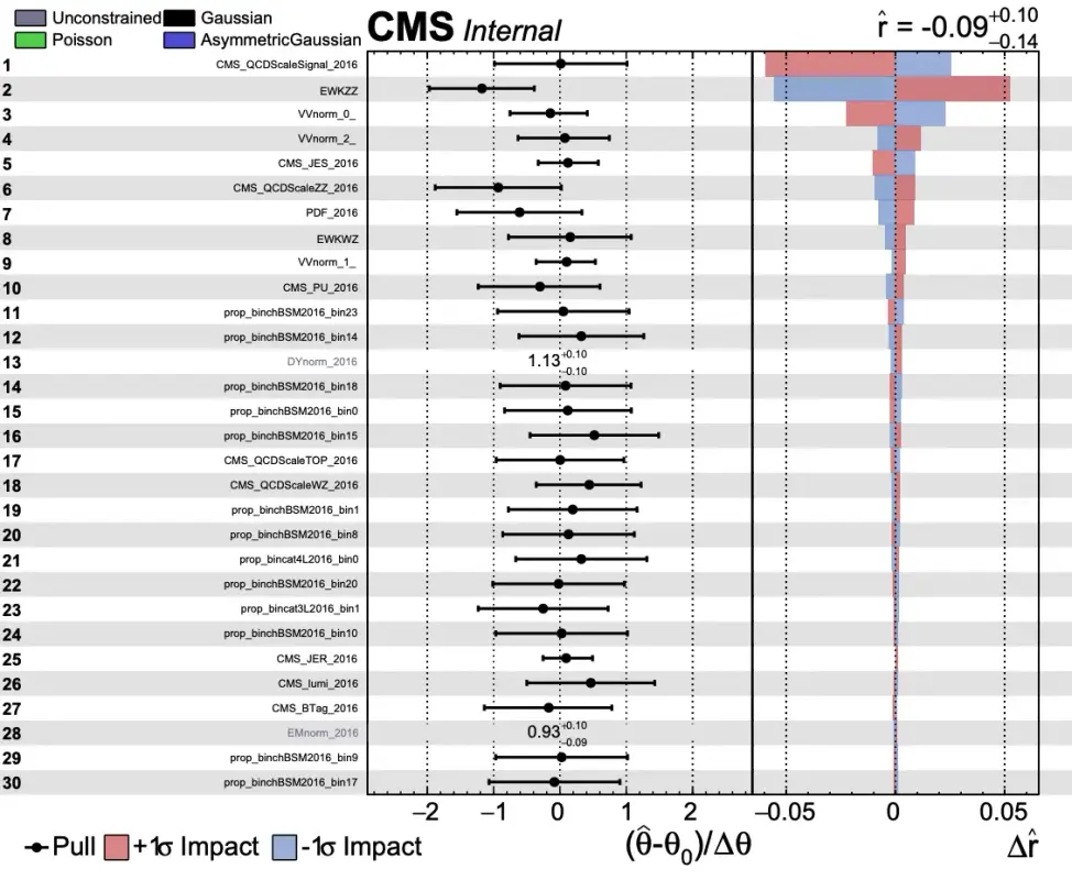
In this sample you can see what a typical impact plot looks like. Here r stands for the signal strength. In the leftmost column you should see a list of various systematic uncertainties (hopefully you will recognize these from the datacards!). The middle column shows the pull values of the uncertainties. This column effectively shows how far off the nominal value combine is using for the fit (if combine were to only use the nominal values then all values here would be 1). The last column is the effect of the systematic uncertainty on the actual signal strength r. If an uncertainty can have a large effect on the signal strength then this delta r value gets larger. This last column takes into account both the up and down fluctuations of the uncertainty. For this plot, the uncertainties are ordered by their effect on the signal strength. There are several more uncertainties than this but only the first page was necessary here as an example.

FitDiagnostics

The next step to try is to look at the fitdiagnostics part of combine. This will form a diagnostics file where you can look at the different ways that we fit the background. The three main categories are:

• prefit (this is without any normalization from combine)
• postfit_b (This is with the normalizations given from combine assuming there is background only)
• postfit_s (This is with the normalizations given from combine assuming there is background and signal)

You can create the diagnostics file using the following command:

combine -M FitDiagnostics workspace_TEST.root -n 'MonoZ' --plots --saveNorm --saveShapes --saveWithUncertainties --saveOverall

This should output a ROOT file named after ‘MonoZ’ in the command above. Now we can look at this ROOT file and see different normalized distributions. Go ahead and explore it a little bit. What processes are available in the file? What about data? We will use this diagnostic file to make some plots in the next section but you should make yourself comfortable with it now.

Running the Limits

To run limits for each signal sample: first copy datacards stored in the following folder including SR and CR for each signal sample: cp -r /eos/user/c/cmsdas/long-exercises/MonoZ/datacards/ for example: cp -r /eos/user/c/cmsdas/long-exercises/MonoZ/datacards/cards-DMSimp_MonoZLL_NLO_Axial_1000_MXd-1/ . we can use following script To create workspace for all signal sample

./make_all_workspaces.sh 

you can find script in creating workspace

This is the bread and butter of the combine tool. Here we will find the limits on the signal samples. This is done with a command like the following:

combine -M AsymptoticLimits --datacard workspace_TEST.root -m 125 -t -1 --name "process name" --rMax=5 --rMin=-10 --cminFallbackAlgo Minuit2,Migrad,0:0.05 --X-rtd MINIMIZER_analytic --X-rtd FAST_VERTICAL_MORPH

Here you need to make sure the process in the workspace_TEST.root is the same as <process name>. This will create limits for this specific sample. There should output like below:

and to generate limits for all signal sample you can use

  ./limit.sh 

<<< Combine >>>
Configured fallback algorithm , type Minuit2, algo Migrad, strategy 0, tolerance 0.05
>>> method used is AsymptoticLimits
>>> random number generator seed is 123456

 -- AsymptoticLimits ( CLs ) --
Observed Limit: r < 0.2752
Expected  2.5%: r < 0.1162
Expected 16.0%: r < 0.1684
Expected 50.0%: r < 0.2754
Expected 84.0%: r < 0.4927
Expected 97.5%: r < 0.8347

Done in 0.03 min (cpu), 0.03 min (real)

The output shown above is quite important! Here the r again represents the signal strength. The respective lines are explained below (not necessarily in the same order):

• Expected 50.0%: This is the expected result if the data matched the MC prediction
• Observed limit: This is the limit attained after unblinding the signal region and testing the data against the prediction
• Expected 16.0% and 84%: These are the plus and minus 1 sigma results for the expected limit
• Expected 2.5% and 97.5%: These are the plus and minus 2 sigma results for the expected limit

Now we have a limit on the signal strength of a DM model! This limit takes into account the data collected at CMS and all the uncertainties related to the collection of that data as well as the uncertainties in the prediction. This is the actual result of the analysis! The next step is to get these for the all of the DM samples available to us. In order to run over all the samples we can use the runcombine.py file here: combine.

This will give output for all of the DM samples available. From here we can make summary plots as discussed in the Results section.

Postfit Plotting

Once we have this FitDiagnostics file from the instructions above we can start to look at the distributions pre-fit and post-fit. Lets do this through the SWAN tool here:

SWAN.

Click on the large link and a menu should appear. The environment is fine as it is naturally configured so hit the “start my session” button. Here you can start new projects and open jupyter notebooks to write code. The advantage of swan is that it is hosted with EOS so we have access to all of our files. You can access your EOS space from lxplus by going to /eos/user/<first letter of username>/<username> (make a symlink to this for easier access). Your projects will appear in the directory SWAN_projects. We will use this tool to do the plotting from this point. You can make new directory for the long exercise and clone the repo here: Github.

To proceed with the next steps, first copy your fitDiagnostics.root file to your EOS area. Then, open that directory within SWAN. If this approach does not work for any reason, an alternative method is to download the fitDiagnostics.root file to your local machine and upload it manually to SWAN. Once the file is available in your SWAN workspace, you may continue with the next instructions

Comparing Postfit

The file we will start with is the CMSDAS_Postfit.ipynb

In this file make sure you connect the correct pathway to your diagnostics file. Then go ahead and execute each of the sections. This is currently configured to look at the 4L control region and then the signal region where we combine the 2 jet categories into a single histogram.

Find these lines:

channel = "cat4L"
#fit_type = "prefit"
fit_type = "fit_b"

Here you can modify the fit type to look at the pre-fit and the post-fit using either background only or background and signal. You can also look at the other categories specifically the 3L and 4L regions. Go ahead and look at these now. How does the pre-fit compare to the post-fit? How is the agreement in the different regions?

---

Introduction

Welcome to the Mono Z page for the CMSDAS Long exercises. These pages will walk you through the Mono Z and give you example code on how the analysis is actually performed.

Introduction on template analysis

What is a template analysis and difference w.r.t. parametric analysis.

To do:

• Access the signal and background TTrees from the directory, Pick any files inside this directory as per your choice :

  /eos/user/c/cmsdas/long-exercises/MonoZ/CMSDAS_NTuples/

• get a signal ttree

• for example you can calculate the number events you expect in 35.9/fb, Nsig, after you apply the cut “2 electrons with pt > 20 “

  "(Electron_pt[0]>20. && Electron_pt[1]>20.)"

• get a background ttree

• calculate number events you expect in 35.9/fb, Nbkg

• from Nsig and Nbkg calculate the expected significance Nsig/sqrt(Nbkg)

• Given a number of data events measured Ndata, how do you measure the signal cross section?

• An example of using this selection is added here Ex1.C

• We can check the number of electrons in each event using:

  Events->Scan("nElectron")

Suggestions:

• You can take a quick look at the missing transverse momentum values for a sampling of events:

  Events->Scan("met_pt")

• Or we can just draw the distribution for this file directly. Does the distribution make sense for this file? Look at another process and see how it differs.

  Events->Draw("met_pt")

• Since in lxplus Draw option is slow, we can dowload any of this file in our local machine and than implement this command to directly draw it. For example:

  scp username@lxplus.cern.ch:/eos/user/c/cmsdas/long-exercises/MonoZ/CMSDAS_NTuples/DarkMatter_MonoZToLL_NLO_Vector_Mx-500_Mv-500_gDM1_gQ0p25_TuneCUETP8M1_13TeV-madgraph/tree_1.root .
  root -l tree_1.root
  Events->Draw("met_pt")

• Number of events we have analysed

  Runs->Scan("genEventSumw")

  You should see an output like below:

  ************************
  *    Row   * genEventS *
  ************************
  *        0 *    895556 *
  ************************

We will learn more about these files and how to use them later but it is good to familiarize yourself with a couple of the processes now. Take some time to look at the MC background, the MC signal and the data separately.

Introduction on Mono-Z analysis

For this analysis we are going to be looking for indications of dark matter (dm) being produced by the LHC. Since dm particles will not be seen by the CMS detector, this means our events with dm would have large amounts of missing transverse momentum (pTmiss). The MonoZ analysis focuses on events with a leptonically decaying Z boson that is recoiling against large amounts of missing transverse momentum. Therefore, the final state consists in two charged leptons of opposite charge, same flavor and reconstruct a mass near the known Z boson mass. Tau leptons are unstable and decay either leptonically (in that case we still have an isolated electron or muon) or hadronically, hence difficult to reconstruct. Therefore, the analysis looks at the final stated with electrons and muons only. Additionally, the signal we are looking for has a low amount of hadronic activity, we will only look at events with 0 or 1 recontrsucted jets. Jets that have been flagged as originating from b quarks will also be rejected in oder to reduce the background from top processes.

In order to look for dm we must understand the SM processes that may produce the same final state of the signal. To categorize of background exist: the irreducible background (ZZ) is due to all the physics processes that generate exactly the same topology of the signal, while the reducible background is due to all those processes that mimic the signal because of faults in the reconstruction. This may happen because of several reasons, typically due to the detector behaviour. For example, hadronic jets may be wrongly identified as charged leptons, or real charged leptons or hadronic jets may not be identified, originating fake MET as if they were neutrinos.

This analysis is a cut and count meaning that we will make selections to try and isolate the signal from the SM background and then used the yield in a binned distribution(s) to calculate the sensitivity and set limits. This twiki will follow the recently published results for Run 2 which can be seen on arXiv here:

arxiv

---

Welcome to the UoH CMSDAS 2025 Tutorial

Select a chapter from the sidebar to begin exploring the mono-Z analysis tutorial.